Can I Make Archos 101 Valid Again

Final Updated on October xiii, 2020

What is a training and testing dissever?Information technology is the splitting of a dataset into multiple parts. We train our model using one function and test its effectiveness on another.

In this commodity, our focus is on the proper methods for modelling a relationship between ii avails.

Nosotros will cheque if bonds tin can exist used every bit a leading indicator for the S&P500.

What is data splitting in modelling?
What is a Training set?
What is a Validation prepare?
What is a Test Set?
Why do we need to split our data?
- Look-ahead Bias
- Overfitting
- Underfitting
How to Train our Model?
How do we use the Validation Set?
Hyper-parameter Tuning with the Validation Set
How do nosotros examination our model on our Testing Set?
What is Cantankerous-Validation and why practise nosotros use it?
Cantankerous-Validation for Standard Information
- K-fold Cantankerous-Validation
- Hyper-parameter Tuning with K-fold Cross-Validation
- Alternative Techniques For Problematic Data
  - Stratified M-fold
  - Group M-fold
Cross-Validation for Fourth dimension Series Information
- Walk-Forward Nested Cross-Validation

What is information splitting in modelling?

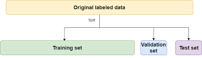
Data splitting is the process of splitting information into iii sets:

Data which we utilize to design our models (Training set)
Information which we use to refine our models (Validation set)
Data which we utilise to test our models (Testing set)

If we do not split our data, we might exam our model with the same data that nosotros apply to train our model.

Example

If the model is a trading strategy specifically designed for Apple stock in 2008, and we test its effectiveness on Apple stock in 2008, of course it is going to do well.

We demand to test it on 2009's data. Thus, 2008 is our training set up and 2009 is our testing set.

To recap what are training, validation and testing sets…

What is a Training Ready?

The grooming set is the set of data we analyse (railroad train on) to blueprint the rules in the model.

A training prepare is also known as the in-sample data or preparation data.

What is a Validation Set?

The validation set is a set of data that nosotros did not use when training our model that nosotros use to appraise how well these rules perform on new data.

Information technology is besides a set we apply to tune parameters and input features for our model and so that information technology gives us what nosotros think is the best performance possible for new data.

What is a Test Set?

The test set is a set up of data we did not apply to railroad train our model or use in the validation gear up to inform our choice of parameters/input features.

We will employ information technology as a last test once we accept decided on our final model, to get the all-time possible estimate of how successful our model will exist when used on entirely new data.

A exam set is besides known as the out-of-sample data or test data.

Why do we need to separate our data?

To prevent wait-ahead bias, overfitting and underfitting.

Look-ahead bias: Edifice a model based on data that is not supposed to be known.
Overfitting: This is the procedure of designing a model that adapts so closely to historical information that it becomes ineffective in the future.
Underfitting: This is the process of designing a model that adapts so loosely to historical data that information technology becomes ineffective in the future.

Await-Ahead Bias

Permit's illustrate this with an example.

Here is Amazon'southward stock performance from 2013 to 2020.

amazon price chart 2013 to 2020 — Source: Tradingview.com

Wow, it is trending up rather smoothly. I'll pattern a trading model that invests in Amazon equally it trends up.

I and then test my trading model on this aforementioned dataset (2013 to 2020).

To my non-surprise, the model performs brilliantly and I make a lot of hypothetical monies. You don't say!

When the trading model is being tested from 2013, it knows what Amazon's 2014 stock behavior will be because we took into business relationship 2014'due south data when designing the trading model.

The model is said to have "looked ahead" into the futurity.

Thus, in that location is look-ahead bias in our model. We built a model based on data we were not supposed to know.

Overfitting

In the simplest sense, when grooming, a model attempts to learn how to map input features (the available data) to the target (what nosotros want to predict).

Overfitting is the term used to describe when a model has learnt this relationship "too well" for the training data.

Past "too well" we hateful rather that it has learnt the relationship also closely- that it sees more trends/correlations/connections than actually exist.

We can call back of this every bit a model picking up on likewise much of the "noise" in the training data- learning to map exact and very specific characteristics of the preparation data to the target when in reality these were one-off occurrences/connections and not representative of the broader patterns more often than not nowadays in the information.

Every bit such, the model performs very well for the training data, only flounders comparatively with new information. The patterns developed from the training data exercise not generalise well to new unseen data.

This is almost ever a consequence of making a model too complex- allowing it to have too many rules and/or features relative to the "real" corporeality of patterns that exist in the data. Its peradventure also a result of having besides many features for the number of observations (preparation data) we have to train with.

For example in the farthermost, imagine we had thousand pieces of training information and a model that had 1000 "rules". It could essentially learn to construct rules that stated:

rule 1: map all data with features extremely close to x1,y1,z1 (which happen to be the exact features of training information 1) to the target value of training data i.
rule ii: map all data with features extremely shut to x2,y2,z2 to the target value of grooming information 2.
…
dominion 1000: map all information with features extremely close to x1000,y1000,z1000 to the target value of preparation information 1000.

Such a model would perform excellently on the training data, but would probably be nearly useless on whatsoever new information that deviated even slightly from the examples that it trained on.

Yous can read more nigh overfitting here: What is Overfitting in Trading?

Underfitting

Past dissimilarity, underfitting is when a model is too non-specific. I.due east., information technology hasn't really learnt any meaningful relationships between the grooming data and the target variable.

Such a model would perform well neither on the preparation information nor whatsoever new data.

This is a rather rarer occurrence in practice than overfitting, and usually occurs because a model is likewise simple- for example imagine plumbing equipment a linear regression model to non-linear data, or maybe a random wood model with a max depth of 2 to data with many features present.

In general you desire to develop a model that captures as many patterns in the training data that exist as possible that nevertheless generalise well (are applicable) to new unseen information.

In other words, we want a model that is neither overfitted or underfitted, but only right.

How to Train our Model

To meet how these concepts play out in reality, lets attempt edifice an actual model.

Our Model: To cheque if yesterday's two-10 Bail Spread tin can predict today's SPX prices.

We will use some information called:

"2-ten Bond Spread" which is the spread between the ten-Yr U.S. Treasury Abiding Maturity rate and the 2-Yr Treasury Abiding Maturity Charge per unit) and
"SPX, SPCFD: Compare" which is a marketplace-capitalization weighted index of the 500 largest U.Southward. publicly traded companies.

Visually our data looks like this:

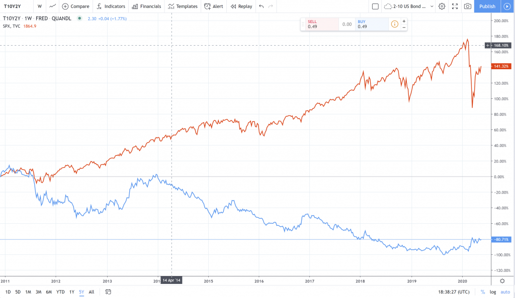
Lets get ahead and load up some instance market data of ii-10y US bond spread against SPX daily close:

            import numpy equally np import pandas every bit pd from pathlib import Path  df = pd.read_csv(Path("QUANDL_FRED_T10Y2Y, 1D 80PERCENT.csv"))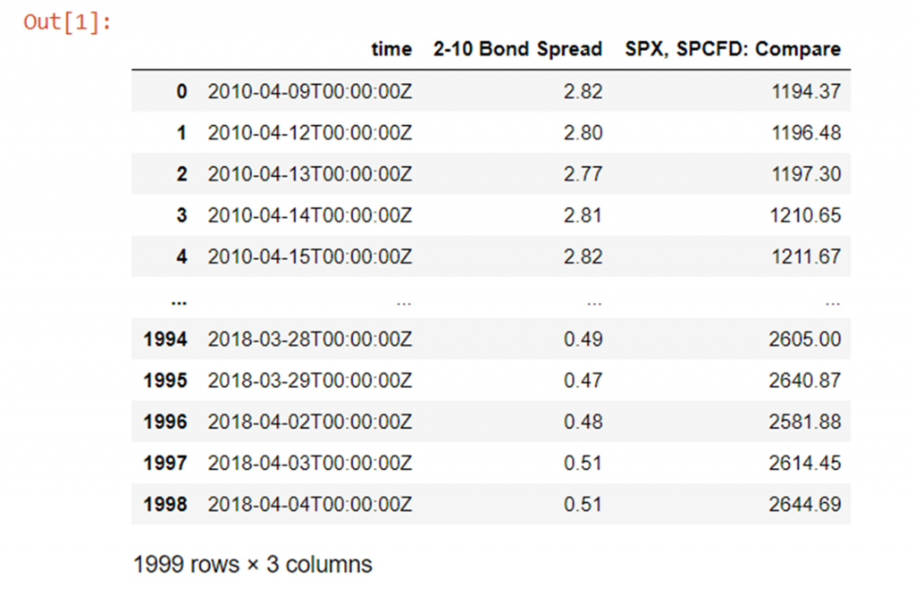

Note that before doing any modelling we will lag the 2-10 US bond spread by 1 mean solar day as we desire to backslide SPX(t) on two-ten(t-1), because as we said we want to check if yesterday's 2-10 value has any issue on today's SPX value. We should also use the returns (proportional price modify from the terminal day) rather than the actual price today.

Shift the bail spread and so that yesterday'southward bond spread is regressed against today's cost:

            df['2-10 Bond Spread'] = df['2-ten Bail Spread'].shift(1)

Regress against (pct) change from yesterday's toll instead of today'due south absolute price:

            df['returns']=df['SPX, SPCFD: Compare']/df['SPX, SPCFD: Compare'].shift(ane) - one df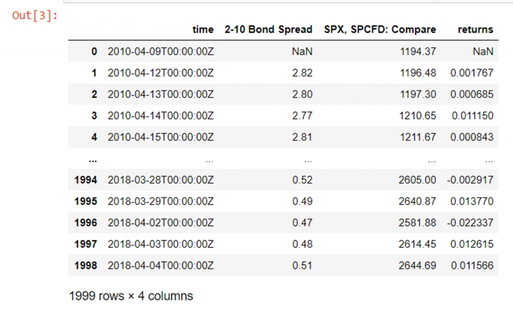

And now clean up a bit by removing the first row which now has an N/A in the "2-10 Bail Spread" and "returns" columns since we shifted "2-10 Bond Spread" up past 1:

            df = df[1:] # remove offset row with an N/A df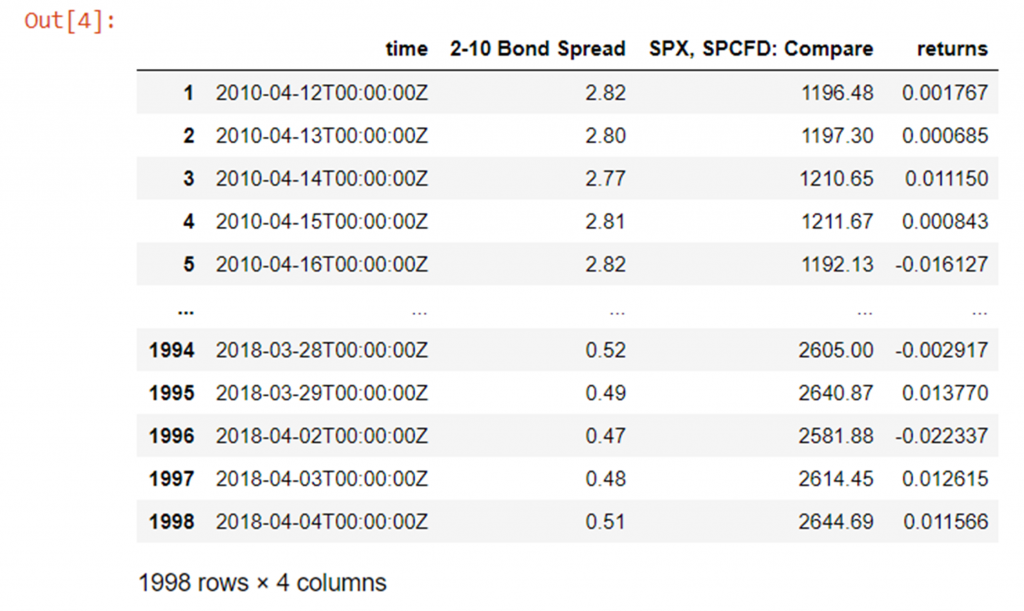

Finally, it would exist convenient to set the alphabetize of the dataframe to the values of the time column instead of arbitrary integers, since the chronology of the data is important.

Note that type of the time column is currently string (you can cheque this yourself with the type(x) part), and so lets set up it first to datetime64 and so set the index to the time column:

            df['time'] = df['time'].astype('datetime64[ns]') # alter "time" cavalcade type from str to datetime64 df.set_index('fourth dimension', inplace=True) # gear up time column as the alphabetize  df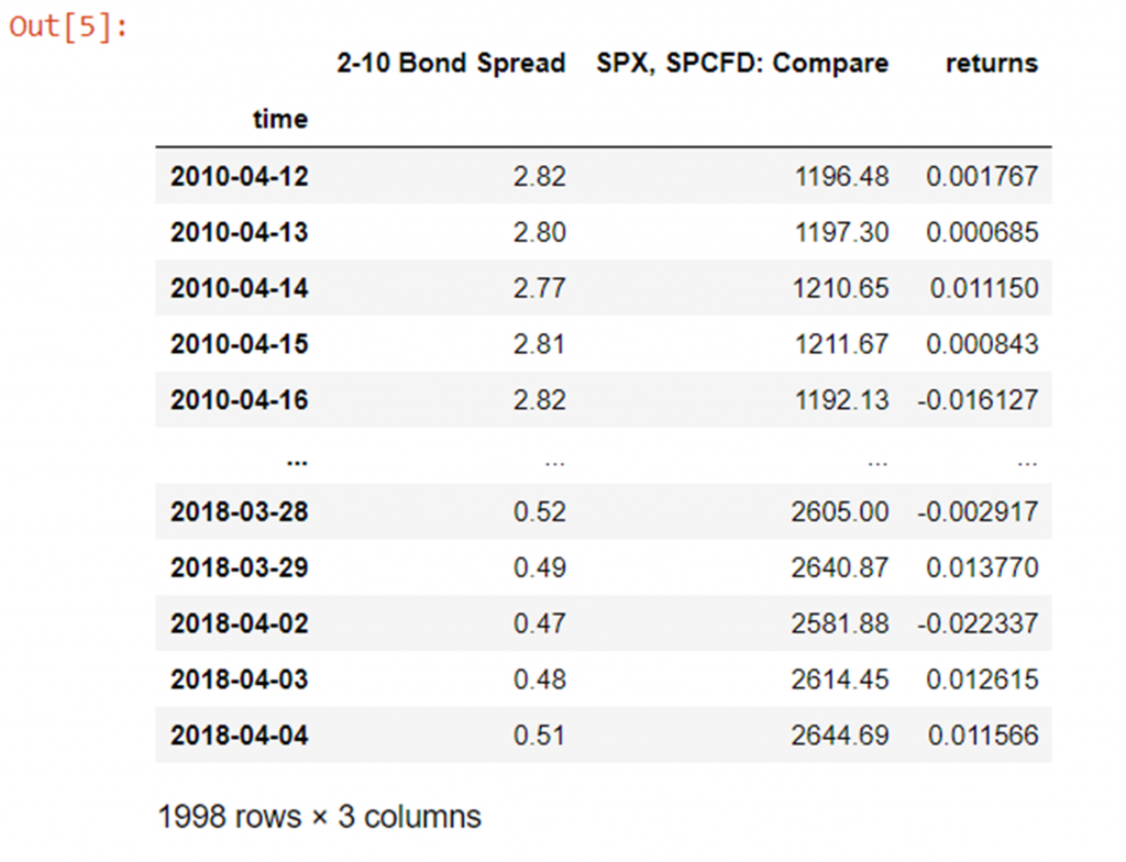

Now lets use all of the data to build our model, and then test our model with the aforementioned data and see what happens.

First lets import from sklearn a very easy to apply regression model for demonstrative purposes, and the mean_squared_error office to help usa generate a root mean squared evaluation function for testing our model:

            from sklearn.ensemble import RandomForestRegressor from sklearn.metrics import mean_squared_error

Note that in sklearn often you lot will find both a "Regressor" and "Classifier" version of the aforementioned algorithm (for instance in this instance RandomForest). You just want to use the classifier version when you are predicting into a finite number of categories (for example equus caballus, shoe, duck) and the regressor version when you lot are attempting to predict a continuous numerical output (as we are here).

At present lets create our training dataframe, and our target dataframe:

            # set the training data columns and target variable y_train = df["returns"] X_train = df.drop(columns=["SPX, SPCFD: Compare", "returns"])

And initialise a RandomForestRegressor with a few hyper-parameter values set. Note that:

random_state just governs the initialisation parameters for the algorithm- if we define it explicitly nosotros volition go completely repeatable results, otherwise it is called randomly and then the terminal model will vary slightly every fourth dimension
max_depth is a variable controlling the depth of the decision copse spawned in the forest- the greater the depth the more splits the model tin can brand on the data- every bit a function of 2^(max_depth) ), allowing the model to grow more than circuitous
n_estimators is the number of individual conclusion trees in the "wood"

            random_forest = RandomForestRegressor(max_depth=5, n_estimators=100, random_state=i)

Lets fit (train) our model on all of our data:

            random_forest.fit(X_train, y_train)

And check the root mean squared accuracy of our fitted model on the same exact same information:

            root_mean_squared_error = np.sqrt(mean_squared_error(y_train, random_forest.predict(X_train))) root_mean_squared_error

          0.009310731251200473

Okay, so we have an error of 0.00931 every bit a baseline operation for our model.

Note that this is pretty horrible since the average return (which yous can calculate with (np.abs(y_train)).mean() ) is 0.0065 and then our boilerplate error is ~143% the size of the average daily return so clearly our model is not very accurate.

This isn't really surprising though since nosotros are using zip but a single numerical value (yesterday's bail spread) and an un-calibrated (and mayhap inappropriate type of) model to estimate the daily render- if markets were actually that piece of cake to predict nosotros would all exist rich!

This doesn't actually matter though and for the purposes of this article we will ignore our objectively horrible results- the focus is on using the dataset to provide demonstrative code for the topics we are exploring, and not the actual skill of our models.

In whatever case nosotros can notwithstanding fiddle with the model hyper-parameters to endeavour and improve our performance.

For instance we tin can increase the max-depth of our random forest (which if we call back allows the model to brand more than splits on the data and thus grow more complex):

            random_forest = RandomForestRegressor(max_depth=10, n_estimators=100, random_state=1) random_forest.fit(X_train, y_train) root_mean_squared_error = np.sqrt(mean_squared_error(y_train, random_forest.predict(X_train))) root_mean_squared_error

          0.009083679274932605

Okay, something like a ~two.4% improvement.

And making it more complex still:

            random_forest = RandomForestRegressor(max_depth=50, n_estimators=100, random_state=1) random_forest.fit(X_train, y_train) root_mean_squared_error = np.sqrt(mean_squared_error(y_train, random_forest.predict(X_train))) root_mean_squared_error

          0.008943288173833334

Almost a 4% improvement now from our beginning point.

Then now that we've improved it a fleck, how does the model perform when exposed to entirely new information?

Hither we will pretend we deployed our model in a live state of affairs, and have come across some new data in the wild. We will load in some more data from the same source (but from a point in fourth dimension moving chronologically forrard from the grooming data) and go through exactly the same pre-processing steps:

            unseen_data = pd.read_csv(Path("unseen_data.csv")) unseen_data['2-10 Bond Spread'] = unseen_data['two-10 Bail Spread'].shift(ane) unseen_data['returns']= unseen_data['SPX, SPCFD: Compare']/unseen_data['SPX, SPCFD: Compare'].shift(1) - 1 unseen_data = unseen_data[1:] unseen_data['time'] = unseen_data['time'].astype('datetime64[ns]') # change "time" cavalcade type from str to datetime64 unseen_data.set_index('time', inplace=True) # set time column equally the alphabetize unseen_data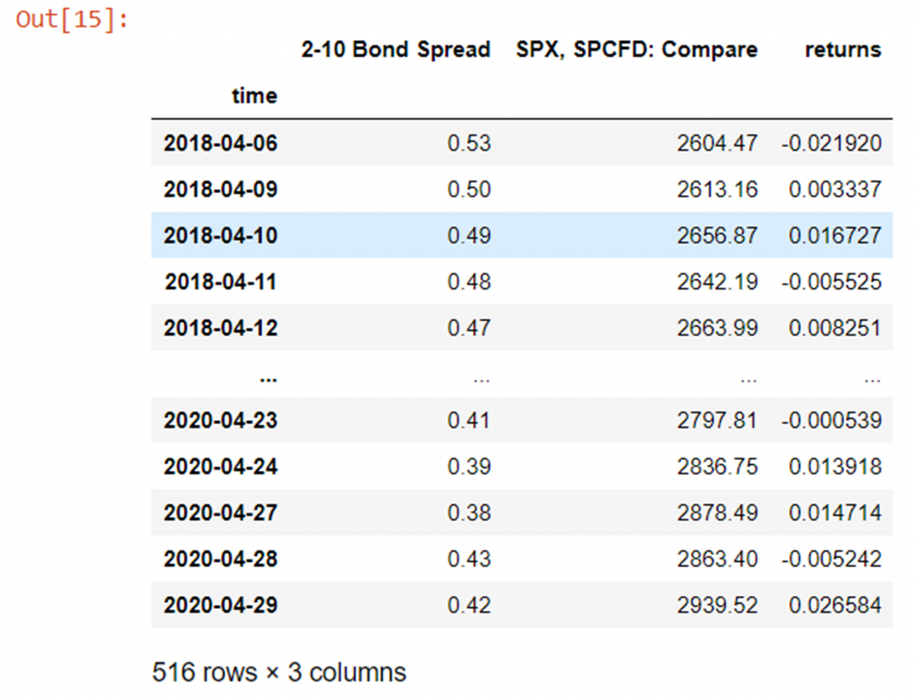

And finally setting the input variable and target variable again and testing our functioning on some new data:

            y_unseen = unseen_data["returns"] X_unseen = unseen_data.drib(columns=["SPX, SPCFD: Compare", "returns"])  root_mean_squared_error = np.sqrt(mean_squared_error(y_unseen, random_forest.predict(X_unseen))) root_mean_squared_error

          0.018704827013423832

Which gives united states a root mean squared error ~two09% as large as for the data we previously used to both railroad train and test on- not nearly as well every bit we might have hoped/expected…

This is a clear sit-in of overfitting in action.

How do we utilize the Validation Set?

And then conspicuously we cannot but employ a model'south performance on it's training data to approximate how well it volition perform on new data.

We demand to gauge it'south performance on some data it did not use to train with to get a better picture of how well it will perform in the wild.

Enter the validation gear up.

From now on nosotros will split our training data into two sets. Nosotros will go on the majority of the data for grooming, just separate out a small-scale fraction to reserve for validation.

A expert rule of thumb is to utilise something effectually an 70:30 to 80:20 training:validation split.

To practice this we could simply do something like circular a specific fraction of the length of our data to an integer and chop our dataframe in 2 as follows:

            y = df["returns"] X = df.drop(columns=["SPX, SPCFD: Compare", "returns"])  train_fraction = 0.8 split_point = int(train_fraction *len(X)) # (len(X) and len(y) are the same anyhow) X_train = Ten[0:split_point] X_valid = Ten[split_point:]  y_train= y[0:split_point] y_valid= y[split_point:]

Or as y'all might see in many places, employ sklearn's useful pre-built train_test_split function equally follows:

            from sklearn.model_selection import train_test_split  X_train, X_valid, y_train, y_valid = train_test_split(X, y, train_size=0.8,test_size=0.2, random_state=101)

Here train_size and test_size are automatically complementary if you only make full out 1, and random_state is a seed for the style the data is split- if you apply the same seed in the future, you will be guaranteed the exact aforementioned information volition be in each of the grooming and validation sets equally earlier.

            print("len(df): {}, split_point: {}, len(X_train): {}, len(X_valid): {}, len(y_train): {}, len(y_valid): {}".format(len(df), split_point, len(X_train), len(X_valid), len(y_train), len(y_valid)))

          len(df): 1998, split_point: 1598, len(X_train): 1598, len(X_valid): 400, len(y_train): 1598, len(y_valid): 400

The validation set essentially allows u.s.a. to check how "overfitted" or "underfitted" our model is.

It allow us to both tune the model complexity to the sweet spot and provides a much meliorate approximate of how the model will perform with unseen information since the model does not use the validation data to train on.

Note that it is entirely normal (even probable) that the validation accuracy volition be lower than the preparation accurateness. In fact, if they were very like, it'd exist a great indicator that your model might not be complex enough (underfitted).

That said the training accuracy doesn't matter.

The only thing that matters is getting the all-time possible validation accuracy, since this is really somewhat reflective of how the model will perform in the wild.

In general increasing model complexity should (randomness aside) almost e'er lead to improved training accuracy, and for a while increasing model complexity volition as well atomic number 82 to improved validation accurateness, every bit the model finds more and better patterns.

Notwithstanding eventually, these patterns will go too specific to the training data and volition not generalise well, so the validation accurateness will beginning to autumn.

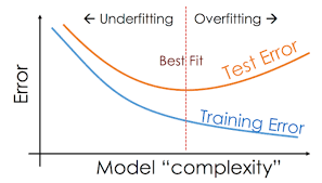
Hyper-parameter Tuning with the Validation Fix

We volition use the validation ready to strop the model's complexity to the sweet spot, as depicted in the image below:

Lets accept a go doing that with our data now.

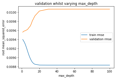
Below we simply iterate over a listing of max_depths, fitting a model to each max depth, then evaluating the mistake on the train and validation sets and making a plot of these. The simply variable we are changing to alter the complexity of the model is the max_depth- everything else remains the same each time- so max_depth is uniquely responsible for the model complexity.

Matplotlib.pyplot is the "standard" plotting library used in Python. Here is a quick crash course in making some uncomplicated plots if you've never encountered information technology before: https://matplotlib.org/tutorials/introductory/pyplot.html

            import matplotlib.pyplot as plt  train_errors = [] valid_errors = [] param_range = [one,2,3,four,v,6,seven,8,9,ten,11,12,13,14,15,twenty,30,40,l,75,100]  for max_depth in param_range:     random_forest = RandomForestRegressor(max_depth=max_depth, n_estimators=100, random_state=1)     random_forest.fit(X_train, y_train)          train_errors.append(np.sqrt(mean_squared_error(y_train, random_forest.predict(X_train))))     valid_errors.append(np.sqrt(mean_squared_error(y_valid, random_forest.predict(X_valid))))       plt.xlabel('max_depth') plt.ylabel('root mean_squared_error') plt.plot(param_range, train_errors, label="train rmse") plt.plot(param_range, valid_errors, label="validation rmse") plt.fable() plt.show()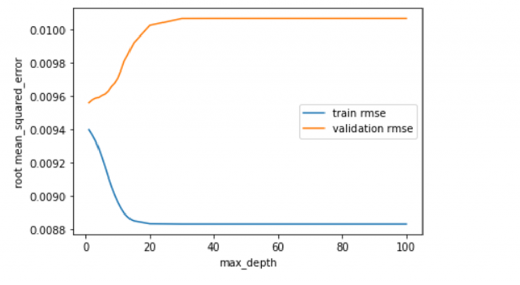

Equally expected we can see that as nosotros increase the max_depth (up the model complexity), the training accuracy continuously improves- speedily at beginning, but still slowly after, throughout the whole i-100 range.

On the other paw the validation accuracy gets worse immediately, and doesn't stop getting worse as we increase the max_depth.

This is an indication that the model is already "also complex" (or at optimal complexity) with a maximum depth of i.

Normally we would expect the validation accuracy to meliorate for at to the lowest degree a piffling while earlier regressing going from a very simple model to very circuitous, but then over again commonly we would expect to use grooming data that contained more than than just a single numeric data column to learn from so a maximum depth of 1 returning the optimal validation functioning is almost certainly just a consequence of very simple input data and/or a lack of training data.

In any example, lets go ahead and re-fit our model with a max_depth of ane and encounter exactly how it performs.

Note that we are reverting to using X and y (the total dataset) here to re-railroad train our model now that nosotros take a theoretical best max_depth so that the grooming data exactly matches that of the first model that predicted against unseen data- chopping off 20% of such a pocket-size dataset (because we recently made a training:validation carve up) would probable crusade our model to perform much worse irrespective of the max depth. This way nosotros proceed the comparison consistent:

            random_forest = RandomForestRegressor(max_depth=1, n_estimators=100, random_state=one) random_forest.fit(X, y) root_mean_squared_error = np.sqrt(mean_squared_error(y, random_forest.predict(X))) root_mean_squared_error

          0.00942170960852716

~five.4% worse than the best we accomplished on the training set when nosotros had a max_depth of l

            root_mean_squared_error = np.sqrt(mean_squared_error(y_unseen, random_forest.predict(X_unseen))) root_mean_squared_error

          0.017679233094329314

Yet ~5.five% better on the unseen information!

Here we have successfully used the validation set to both:

Give us a better advanced estimate of how nosotros will perform on unseen data.
Improve our operation on out of sample (unseen) data by reducing overfitting/underfitting.

How do we test our model on our Testing Set?

So if the model never trains on the validation information, isn't the validation data a perfect gauge of how the model volition perform in the wild?

Well almost.

Just not quite.

The reason is that by using the validation data to tune our model to the best generalisable performance, nosotros have inherently shown a slight bias towards model hyperparameter values and data features that optimise functioning specifically for this validation ready.

In upshot we accept overfitted to the validation set up.

Notation that the degree of overfitting to this set compared to the preparation data is far smaller, and the performance on the validation set will often give a rough ballpark for operation in the wild (bold you have created the validation fix without information leakage- more on that afterward!).

It is for this reason though that nosotros separate out from our available data a farther examination set that nosotros do not touch until we have the final version of our model fully feature-engineered and tuned.

Making this additional split, our original available data should now look something like this:

And nosotros might utilise something similar a 70:twenty:x split now. Nosotros tin can use any way we like to dissever the information-frames, just one choice is merely to use train_test_split() twice.

Note that 0.875*0.8 = 0.vii and then the last effect of these two splits is to take the original data split into training/validation/test sets in a 70:twenty:ten ratio:

            # split the full data 80:20 into training:validation sets X_train, X_valid, y_train, y_valid = train_test_split(X, y, train_size=0.viii, random_state=101)  # split grooming data 87.five:12.five into training:testing sets X_train, X_test, y_train, y_test = train_test_split(X_train, y_train, train_size=0.875, random_state=101)  print("len(X): {} len(y): {} \nlen(X_train): {}, len(X_valid): {}, len(X_test): \ {} \nlen(y_train): {}, len(y_valid): {}, len(y_test): {}".format(len(X), len(y),\ len(X_train), len(X_valid), len(X_test), len(y_train), len(y_valid), \ len(y_test)))

          len(Ten): 1998 len(y): 1998  len(X_train): 1398, len(X_valid): 400, len(X_test): 200  len(y_train): 1398, len(y_valid): 400, len(y_test): 200

We tin can spend as much time and endeavour trying to optimise our performance on the validation set equally we want.

Only we accept to be honest ourselves- when we are done we are done, and must take whatever issue we then go on the testing set as our probable upshot on new information in the wild.

Nosotros cannot then proceed and effort to optimise again to improve the performance farther on the testing set. To practise so would be developing overfitting bias all over again.

What is Cross-Validation and why practise we employ information technology?

Great, then we now split up our data in three ways- we utilise the bulk of our data for training, keep a reasonable amount for validation and proceed a further modest concord-out set for final testing.

But yous might be thinking, aren't we at present losing a lot of data nosotros could exist using for training? Won't this potentially lower our model accurateness?

Also, is there any fashion nosotros can avoid overfitting so much to the validation set?

Well the answer to all 3 questions is yes!

Instead of using a single validation gear up, nosotros tin can apply many validation sets.

We tin can make many training:validation splits and cycle which part of the data we utilise for validation each time such that eventually, over every preparation:validation separate combined, all the data has been used at to the lowest degree one time for validation, and at least once for preparation.

The way in which cross-validation is performed differs for standard and time-series information, but in general gives the states the following benefits:

We get to (over multiple splits) employ 100% of the training + validation data for grooming, which smooths out issues where the initial preparation set was possibly highly biased and contained many examples of an extreme data type/occurrence, or did not contain whatsoever examples of an important data blazon/occurrence
Nosotros become to (piece-wise) validate over all of the data: not falling casualty to any instances of high variance in the small validation prepare where equally the validation set up contained an unusually loftier or low count of unusual occurrences.
We become to boilerplate our performance over all of the data, giving united states far more confidence in our estimation of the model's skill, besides as an actual moving-picture show of how volatile the model is to perturbations in the input data.
Nosotros are automatically forced to build a far less overfitted (and thus more generalisable model) because we are trying to maximise the average operation over many validation sets, not i specific validation ready, so nosotros cannot inadvertently tune towards hyper-parameter settings that are only good for a very specific validation prepare.

Cross-Validation for Standard Information

There are a few different ways we can perform cross-validation, but for non-time series data one of the almost popular (and simple to understand and effective) techniques is K-fold cross-validation.

Note that information technology is true that we have time-serial data here, so K-fold cross validation is actually an inappropriate technique to use (for reasons we shall discuss shortly) only for now nosotros will temporarily ignore these bug for the sake of generating some example lawmaking with the same dataset.

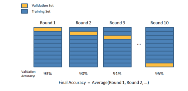
M-fold Cross-Validation

With 1000-fold cantankerous-validation we split the preparation data into k equally sized sets ("folds"), accept a single set as our validation set and combine the other set as our training set up. We then bicycle which fold nosotros utilise as our validation set until we have trained and validated k times- each time with a unique train:validation split up.

You can pick whatever value of k you like, only from the collective experience of all data scientists ever, g=5 or k=x (and everything in between) are mutual and effective choices: grand=5 would correspond an lxxx:xx training:validation carve up and k=10 a 90:10 split etc.

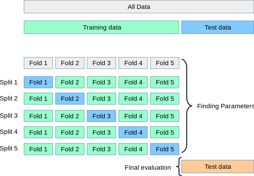
The process tin can exist summarised as follows:

Carve up out from the information a final holdout testing set (perhaps something like ~10% if we have a good amount of data).
Shuffle the remaining data randomly.
Split this data into grand equally sized sets/folds.
For each unique fold:
1. Use this fold equally the validation fold
2. Combine the other k-1 folds as the training data
3. Fit the model with the training information
4. Evaluate the model with the validation fold
5. Proceed the evaluation scores, discard the model and brainstorm over again at 4.one with a new validation fold
Evaluate your model against the whole set of k validation scores, and if you are unhappy make adjustments and repeat from 1.
When you are finally happy, combine all k folds into one complete training data set, train again, and perform a final test on the holdout testing set.

Pictorially the procedure looks something like this:

Visual representation past Joseph Nelson- @josephofiowa

And and so at present the overall training/validation/testing carve up process looks similar this:

https://scikit-learn.org/stable/modules/cross_validation.html

Lets accept a go at attempting to incorporate G-fold cantankerous-validation with our data set up!

While we could write a lot of (unproblematic, but lengthy) lawmaking to implement such a procedure from scratch, luckily the sklearn library comes to our rescue with a handy pre-built office once over again! (y'all can read more nigh information technology here: https://scikit-learn.org/stable/modules/cross_validation.html )

            from sklearn.model_selection import cross_val_score

This magic function is going to handle the whole process very easily for us but practise dig into the documentation to understand how it works under the hood and the variations available!

Anyhow, lets pass the cross_val_score() office our model with our desired parameters, the X and y data (which should be all of the information minus the terminal holdout test set), a scoring method (we will use neg_mean_squared_error and adjust to subsequently to RMSE), and the value of k to use (which is the "cv" parameter):

            cross_val_scores = cross_val_score(RandomForestRegressor(max_depth=one, n_estimators=100, random_state=1),\                                    X, y, scoring='neg_mean_squared_error', cv=5)

Adjust the scores from negative hateful squared fault to root hateful squared error to be consistent with our scores from before:

            cross_val_scores = np.sqrt(np.abs(cross_val_scores))  impress(cross_val_scores) print("mean:", np.hateful(cross_val_scores))

          [0.01360711 0.00861119 0.00715738 0.00947426 0.0067502 ] mean: 0.009120025719774182

As you can run across in that location is huge fluctuation in our validation scores for unlike training:validation splits! The worst error is ~102% greater than the smallest!

These crazy differences are probably mainly a function of our dataset being besides small, and the fact that Thou-fold cross validation is non advisable for time serial data (so some of our training:validation splits might randomly be more appropriate than others) but it goes to highlight that performance can vary quite strongly from split to split so information technology is important to take an average over all the models/splits where eventually all the data is used to validate once!

Note as a sit-in of the fact that very small validation sets pb to high variance (because the small corporeality of information independent in them is subject field to changing a lot with each split up), we can ready grand=50 and run our cantankerous-validation again:

            cross_val_scores = cross_val_score(RandomForestRegressor(max_depth=one, n_estimators=100, random_state=1),\                                    X_train, y_train, scoring='neg_mean_squared_error', cv=50)  # alter neg_mean_squared error to mean_squared_error cross_val_scores = np.sqrt(np.abs(cross_val_scores))  print(cross_val_scores) print("mean:", np.mean(cross_val_scores))

          [0.01029598 0.00922735 0.00553913 0.00900553 0.0110392  0.01333214  0.0115197  0.00933864 0.00664628 0.004857   0.0135743  0.00595552  0.00706495 0.00944506 0.01080077 0.00842491 0.01044174 0.0126128  0.00869932 0.00846706 0.00762137 0.01478009 0.00772207 0.01305496  0.00673948 0.00801689 0.01060272 0.01137826 0.0069177  0.01071186  0.0083437  0.00905157 0.00803609 0.00893249 0.01002789 0.00802375  0.00934506 0.01199787 0.00686557 0.01114371 0.00862676 0.00830973  0.00935762 0.00815328 0.00868262 0.00938199 0.00926949 0.00627161  0.00922161 0.00771521] mean: 0.00921180787871304

Notice how the hateful is very similar, simply the variance is even greater- with the worst functioning having an error ~204% greater than the best!

This is why we like to pick a value of thou somewhere between 5 and ten: the validation sets are big enough not to show too much set to set variance, yet not so big that they take away a substantial clamper of the preparation data- leading to high bias in the grooming information set and a lack of data left over for training.

Hyper-parameter Tuning with Yard-fold Cross-Validation

So as y'all may think, 1 of the points of cross-validation was to reduce bias in the training set, and variance in the validation set.

The other big one was to reduce overfitting to the validation set by forcing us to find hyper-parameter values that give the best average performance over many validation sets.

Before we found that for our specific preparation:validation carve up, a max_depth of 1 led to the best performance, so we concluded that this max_depth would give us the best performance on new data.

Lets remind ourselves of how that looked:

That said its entirely possible that a max_depth of one was but best for this specific validation prepare- it is peradventure not the all-time max_depth averaged over many validation sets.

Lets run hyper-parameter scale for max_depth once more, but this fourth dimension calibrated with cantankerous-validation over 5 different validation sets.

For this we volition use some other function from sklearn- validation_curve ().

            from sklearn.model_selection import validation_curve

It'southward pretty similar to cross_val_scores(), but lets us vary hyper-parameters at the same time as running cross-validation (i.eastward. information technology performs the full cross-validation procedure one time with each specific value of the hyper-parameter we are varying):

            train_scores, valid_scores = validation_curve(RandomForestRegressor(n_estimators=100, random_state=ane), X_train, y_train, "max_depth",                                                param_range, scoring='neg_mean_squared_error', cv=5) train_scores = np.sqrt(np.abs(train_scores)) valid_scores = np.sqrt(np.abs(valid_scores))  train_scores_mean = np.mean(train_scores, centrality=1) valid_scores_mean = np.mean(valid_scores, centrality=i)  plt.title("Validation Curve with Random Woods") plt.xlabel("max_depth") plt.ylabel("RMSE") plt.plot(param_range, train_scores_mean, characterization="train rmse") plt.plot(param_range, valid_scores_mean, characterization="validation rmse")  plt.fable() plt.show()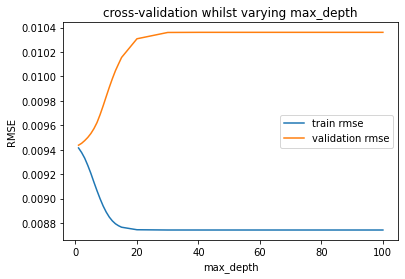

Okay, pretty much exactly the same consequence, but this time around nosotros are much more sure we made a adept choice!

In general, if our data had been a bit more complex and the overfitting with whatsoever level of max_depth wasn't so clear cut, nosotros might find different hyper-parameters gave the best result when varied with cantankerous-validation rather than with validation on a unmarried set.

Alternative Techniques For Problematic Data

K-fold cantankerous validation volition often give y'all a expert event, but occasionally depending on the structure/distribution of the information it tin can give us problems.

The kickoff of these is in the case that there are a lot of extreme examples in the data and nosotros do not go a good distribution of them between the training, validation and testing sets.

For example there could exist few examples of some classes in a classification task. If these (past bad luck) end upwardly mainly merely in the validation or testing sets, then our model volition take never/barely encountered them in training and volition almost certainly perform badly in classifying them.

Similarly in a regression sense, if there are some examples of very extreme target values- either depression or high- and they simply plough up in some of our validation and testing sets, again our model is unlikely to do well when encountering them.

Additionally, if "problematic" information merely appears in the training, and doesn't evidence up in our testing set, we are likely to get an overly optimistic estimation of our model skill- we would like the preparation/validation/testing distributions to be equally similar as possible.

Stratified Thousand-fold

Stratified G-fold is a skilful solution to this.

Information technology's a variation of k-fold which places approximately the same pct of samples of each target class as in the consummate data fix in each of the training, validation and testing sets.

Yous tin import and fix information technology up like so:

            from sklearn.model_selection import StratifiedKFold skfold = StratifiedKFold(n_splits=5, shuffle=Truthful, random_state=1)

Note that information technology returns the indexes of the training/testing (or preparation/validation) splits yous should utilize, so you volition have to manually configure your splits each time as follows:

            for train_index, test_index in skfold.divide(Ten, y): 	X_train, X_test= 10[train_index], 10[test_index] 	y_train, y_test= y[train_index], y[test_index]    # TRAIN AND VALIDATE WITH THIS Dissever

Stratified G-fold only works for classification data direct out of the box, but a sneaky and easy way to become information technology to accept a similar effect for regression data is just to bin your regression targets into narrow-ish bands turning the trouble into pseudo-classification.

Yous could even temporarily add a new column to your data equal to the binned target values, assign this temporary column every bit the target variable, create your "stratified" folds based on this, then drib this extra data column you created and revert to using the exact numeric values as the target variable for the actual training, validation and testing.

Group-K-fold

Another possible issue is when at that place is obvious group structure nowadays in the data.

For example we could have a scenario where samples of information are collected from different subjects, simply in some (or all) cases multiple samples are collected per subject.

Recollect mayhap of trying to estimate how long containers unloaded from cargo ships dwell in dockyards before leaving a terminal. Each send might unload hundreds of containers, so in that location is an obvious grouping of container information long term by ship. If the model is flexible plenty to acquire highly transport-container specific features, information technology could fail to generalise well to containers unloaded from dissimilar ships in the future, fifty-fifty if it performs very well over a grooming/validation/testing split made from containers coming from the same ship.

GroupKFold is a variation of Grand-fold which ensures that the same grouping is not represented in the different sets- i.e. that all instances of data coming from the aforementioned group are present only in one of either the training, validation or testing sets.

You lot tin can use it in exactly the same way every bit StratifiedKfold:

            from sklearn.model_selection import GroupKFold  10 = [0.1, 0.2, two.2, 2.4, ii.3, 4.55, 5.eight, eight.8, ix, x] y = ["a", "b", "b", "b", "c", "c", "c", "d", "d", "d"] groups = [1, ane, ane, 2, 2, two, three, 3, 3, 3]  gkf = GroupKFold(n_splits=iii)  for railroad train, test in gkf.split up(X, y, groups=groups):     impress("TRAIN INDEXES: {} Test INDEXES: {}".format(train, test))

          TRAIN INDEXES: [0 i two three iv 5] Test INDEXES: [6 vii 8 ix] TRAIN INDEXES: [0 1 2 vi 7 8 nine] Examination INDEXES: [3 4 5] Train INDEXES: [iii 4 5 6 7 8 9] Examination INDEXES: [0 1 2]

As y'all can encounter data from each group appears completely in either the training set or testing set for each separate.

Cross-Validation for Fourth dimension Series Data

1000-fold cross validation (and it's variants) work poorly for time series data because they do non respect the chronological ordering of the data.

The data that goes into each of the grooming, validation and testing splits is picked randomly so we will nigh invariably take some corporeality of the preparation data come up before as well every bit after the validation and testing sets.

If the patterns in the information are highly dependant on the fourth dimension they occurred as well as their other features, then essentially this is a form of information leakage as we are using some information from the future to predict the past and present leading to overly optimistic estimates of model skill.

This can exist a disaster in some situations as in certain situations it is much easier to fill in the bare about some middling time event if given information from before and subsequently it.

For case think markets- a million dollar question (or trillion?) to predict how they will move in the future with information from the present, but rather easier to guess what happened in terms of toll movements in the middle of given time range if given price data from before and afterwards the menses of question (especially on a depression time frame).

Note that the explicit presence of a time of data observation column in your information doesn't necessarily forcefulness the definition of whether some data should be considered as a time series or not. It is possible to have an observed time cavalcade in your data and for the data to not be strongly time dependant- you have to consider the nature of the data.

For instance, how human bone measurements correlate to tiptop probably has varied slightly over the millennia, but over a period of years or even decades, time is not a strongly relevant component, even if yous have the time of observation in your data. Market toll movements on the other hand, are highly sensitive to time- even down to the minutes and seconds.

Because of this, for fourth dimension serial data it is essential that the testing prepare is composed of data strictly from chronologically afterwards the validation and training sets, and as well that the validation information comes chronologically after the preparation gear up.

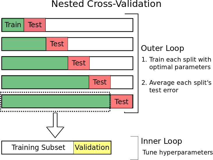
Walk-Forward Nested Cross-Validation

To achieve this whilst still being able to use the majority of our data for validation (and testing also as it turns out in this instance), we tin utilise a technique known as walk-foward nested cross-validation.

The idea is pretty simple.

Nosotros begin using but a small-scale fraction of our information in the past.

We then:

Utilise the nigh contempo information in that set as our test data
Use the information merely prior to that as the validation set
Use all the data prior to that every bit our preparation fix
Aggrandize our data gear up forward in time and repeat 1-three until the data in our exam set catches up to the present twenty-four hours.

The procedure should look something like this:

Courtney Cochrane: https://towardsdatascience.com/time-series-nested-cross-validation-76adba623eb9

Whilst that might look technically catchy to implement, sklearn has (unsurprisingly) some other useful part to assist us out with this- TimeSeriesSplit().

            from sklearn.model_selection import TimeSeriesSplit

Starting time, do make certain your data-frame has it's index set up as the relevant time serial (nosotros already did this right at the start) to make sure the index is chronologically ordered.

And so create a TimeSeriesSplit() object with the amount of walk-forrad splits you want (north=five gives v walk-foward cycles with equal sized test sets):

            tscv = TimeSeriesSplit(n_splits=5)

When used on a dataframe tscv returns the indexes of the training:test splits in a generative fashion.

Below I've created some simpler data to show the output so that it's easier to tell whats going on:

            X = np.array([[1, 2], [iii, iv], [ane, two], [3, 4], [1, 2], [3, 4],[i, 2], [iii, four], [i, 2], [3, four]]) y = np.array([1, 2, three, four, 5, 6, 7, 8, nine, 10])  for train_index, test_index in tscv.split(Ten):     print("Train:", train_index, "TEST:", test_index)     X_train, X_test = X[train_index], X[test_index]     y_train, y_test = y[train_index], y[test_index]

          TRAIN: [0 1 2 3 four] Exam: [5] Railroad train: [0 1 2 3 4 5] TEST: [6] Railroad train: [0 1 two 3 4 v 6] Test: [vii] TRAIN: [0 1 2 three 4 5 half dozen vii] TEST: [8] Train: [0 i 2 iii four 5 6 7 viii] Exam: [9]

This gives us our walk-forrard preparation:testing divisions beautifully.

We tin can now but chop off whatever fraction nosotros like by index of the final information in the train set up in each walk-forward example to grade the validation data, since it is chronologically ordered by our time series index anyway:

            for train_index, test_index in tscv.split(X):     # eighty:xx training:validation inner loop split     inner_split_point = int(0.eight*len(train_index))          valid_index = train_index[inner_split_point:]     train_index = train_index[:inner_split_point]      print("TRAIN:", train_index, "VALID:", valid_index, "TEST:", test_index)          X_train, X_valid, X_test = X[train_index], X[valid_index], Ten[test_index]     y_train, y_valid, y_test = y[train_index], y[valid_index], y[test_index]

          Railroad train: [0 one 2 3] VALID: [4] TEST: [5] TRAIN: [0 i two iii] VALID: [4 v] TEST: [6] TRAIN: [0 1 2 3 4] VALID: [v six] TEST: [7] Railroad train: [0 one 2 3 4 5] VALID: [6 7] TEST: [viii] TRAIN: [0 1 2 iii 4 5 6] VALID: [vii eight] Examination: [9]

Perfect! (though do note we need just a few data samples relative to the size of n_splits to guarantee all non-empty sets- but this is inappreciably likely to be a problem in reality!)

At present we can simply perform training and validation in a single set (non cross-validation) manner each fourth dimension in the inner loop. We won't go through this with an example again since it tin can be performed exactly as in the Hyper-parameter Tuning with the Validation Set department.

Notation as a final betoken, once you have gone through your chosen variation of training, cross validating and testing your model, it is worth combining all three of your training, validation and testing sets and retraining ane final time before heading into the wild.

This final recombination maximises the amount of information the model tin acquire from (now that we take the optimal features and hyper-parameter settings already figured out) and so will probably lead to a slightly more than effective and robust model!

Hopefully this article has given you a few new ideas to play around with and reinforced your understanding of the why behind training, validation and testing sets.

You tin discover the code used in this article and the accompanying datasets hither: https://github.com/GregBland/train_val_test_sets_article

Until the side by side time!

Related commodity: What is a Walk-Forward Optimization and How to Run It?

gordonflunhat84.blogspot.com

Source: https://algotrading101.com/learn/train-test-split/